2. Loading Data
import networkx as nx
2.1. Formats
2.1.1. Adjacency List
If the data is in an adjacency list, it will appear like below. The left most represents nodes, and others on its right represents nodes that are linked to it.
0 1 2 3 5
1 3 6
2
3 4
4 5 7
5 8
6
7
8 9
9
To call it from a file, we use nx.read_adlist.
G2 = nx.read_adjlist('G_adjlist.txt', nodetype=int)
G2.edges()

[(0, 1),
 (0, 2),
 (0, 3),
 (0, 5),
 (1, 3),
 (1, 6),
 (3, 4),
 (5, 4),
 (5, 8),
 (4, 7),
 (8, 9)]
2.1.2. Edge List
Edge list is just a two column representation of one node to another. It can have additional columns for weights.
[(0, 1, {'weight': 4}),
 (0, 2, {'weight': 3}),
 (0, 3, {'weight': 2}),
 (0, 5, {'weight': 6}),
 (1, 3, {'weight': 2}),
 (1, 6, {'weight': 5}),
 (3, 4, {'weight': 3}),
 (5, 4, {'weight': 1}),
 (5, 8, {'weight': 6}),
 (4, 7, {'weight': 2}),
 (8, 9, {'weight': 1})]
We can use nx.read_edgelist() to transform it into a graph network.
G4 = nx.read_edgelist('G_edgelist.txt', data=[('Weight', int)], delimiter='\t')
For multiple edge attributes and graph definition, we have addition definitions in the read_edgelist() function.
chess = nx.read_edgelist('chess_graph.txt', data=[('outcome', int), ('timestamp', float)],
                         create_using=nx.MultiDiGraph())
2.1.3. Adjacency Matrix
From a graph network, we can transform it into an adjacency matrix using a pandas dataframe.
import pandas as pd

nx.to_pandas_dataframe(g, weight='distance')

      1.0         2.0     3.0     4.0     5.0   6.0       7.0
1.0     0.0           1306.0  0.0         0.0   2161.0        2661.0  0.0
2.0     1306.0        0.0         919.0         629.0 0.0         0.0     0.0
3.0     0.0       919.0         0.0       435.0       1225.0  0.0         1983.0
4.0     0.0       629.0         435.0   0.0     0.0       0.0     0.0
5.0     2161.0        0.0         1225.0      0.0       0.0       1483.0      1258.0
6.0     2661.0        0.0         0.0     0.0   1483.0        0.0         0.0
7.0     0.0       0.0     1983.0      0.0     1258.0  0.0     0.0
An adjacency matrix can also be loaded back to a graph
G3 = nx.Graph(matrix)
G3.edges()
2.2. Pickle > Graph
G = nx.read_gpickle('major_us_cities')
2.3. SQL > DataFrame > Graph
The below code uses an edge list format.
import psycopg2
import pandas as pd

conn = psycopg2.connect(database="postgres", user="postgres", password="***", host="127.0.0.1", port="5432")

query = """SELECT fromnode, tonode, distance from edges"""
df = pd.read_sql_query(query, conn)
g = nx.from_pandas_dataframe(df, 'fromnode', 'tonode', 'distance') # or edge_attr='distance'
2.4. Graph > DataFrame
Sometimes, it is necessary to convert a graph into an edge list into a dataframe to utilise pandas powerful analysis abilities.
df = pd.DataFrame(new.edges(data=True), columns=['name1','name2','weights'])
Note that weight attributes are in a dictionary.
name1   name2   weights
Georgia       Lee         {u'Weight': 10}
Georgia       Claude  {u'Weight': 90}
Georgia       Andy      {u'Weight': -10}
Georgia       Pablo     {u'Weight': 0}
Georgia       Frida     {u'Weight': 0}
Georgia       Vincent {u'Weight': 0}
Georgia       Joan      {u'Weight': 0}
Lee       Claude      {u'Weight': 0}
But we can easily extract the dictionary value using a map function.
df['relation'] = df['weights'].map(lambda x: x['Weight'])
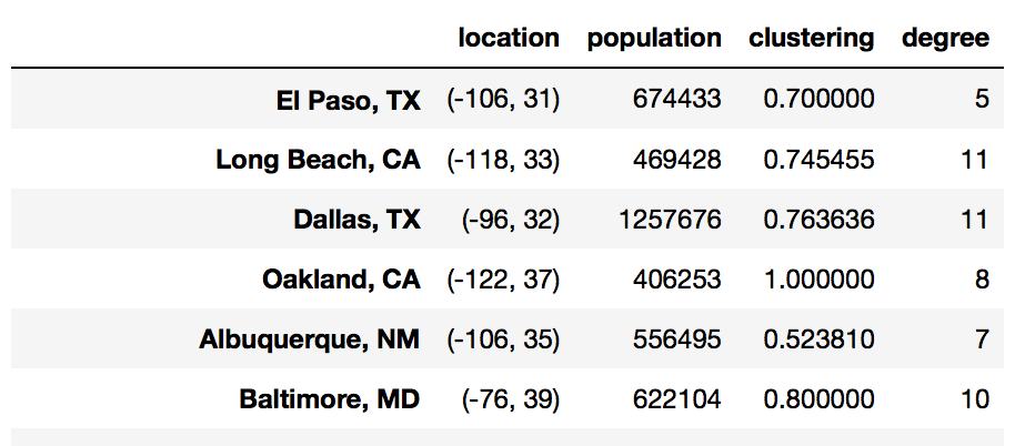
To extract node attributes into dataframe
G.nodes(data=True)
#  [('El Paso, TX', {'location': (-106, 31), 'population': 674433}),
# ('Long Beach, CA', {'location': (-118, 33), 'population': 469428}),
# ('Dallas, TX', {'location': (-96, 32), 'population': 1257676}),
# ('Oakland, CA', {'location': (-122, 37), 'population': 406253}),
# ('Albuquerque, NM', {'location': (-106, 35), 'population': 556495}),
# ('Baltimore, MD', {'location': (-76, 39), 'population': 622104}),
# ('Raleigh, NC', {'location': (-78, 35), 'population': 431746}),
# ('Mesa, AZ', {'location': (-111, 33), 'population': 457587})....

# Initialize the dataframe, using the nodes as the index
df = pd.DataFrame(index=G.nodes())

df['location'] = pd.Series(nx.get_node_attributes(G, 'location'))
df['population'] = pd.Series(nx.get_node_attributes(G, 'population'))
Most of the networkx functions related to nodes return a dictionary, which can also easily be added to our dataframe.
df['clustering'] = pd.Series(nx.clustering(G))
df['degree'] = pd.Series(G.degree())
From University of Michigan, Python for Data Science Coursera Specialization
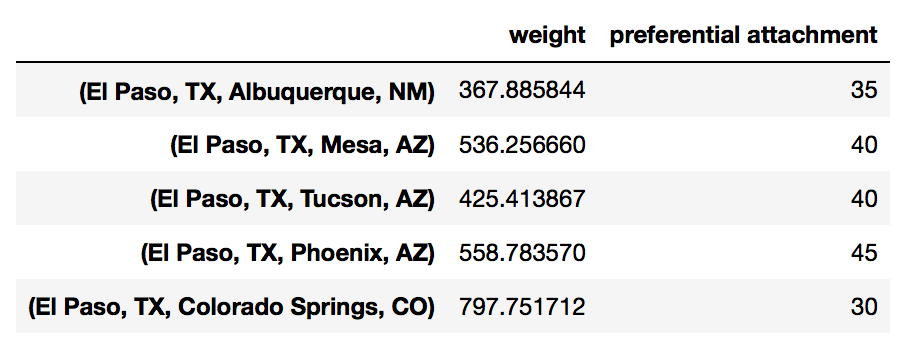
To extract edge features into dataframe
# Initialize the dataframe, using the edges as the index
df = pd.DataFrame(index=G.edges())
# [('El Paso, TX', 'Albuquerque, NM', {'weight': 367.88584356108345}),
#  ('El Paso, TX', 'Mesa, AZ', {'weight': 536.256659972679}),
#  ('El Paso, TX', 'Tucson, AZ', {'weight': 425.41386739988224}),
#  ('El Paso, TX', 'Phoenix, AZ', {'weight': 558.7835703774161}),
#  ('El Paso, TX', 'Colorado Springs, CO', {'weight': 797.7517116740046}),
#  ('Long Beach, CA', 'Oakland, CA', {'weight': 579.5829987228403})....

df['weight'] = pd.Series(nx.get_edge_attributes(G, 'weight'))
Many of the networkx functions related to edges return a nested data structures. We can extract the relevant data using list comprehension.
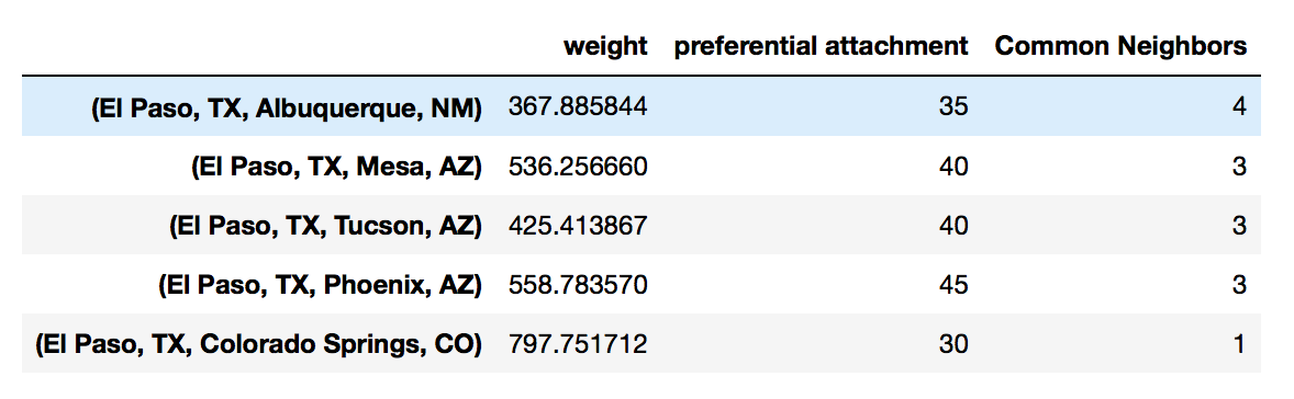
df['preferential attachment'] = [i[2] for i in nx.preferential_attachment(G, df.index)]
From University of Michigan, Python for Data Science Coursera Specialization
In the case where the function expects two nodes to be passed in, we can map the index to a lamda function.
df['Common Neighbors'] \
= df.index.map(lambda city: len(list(nx.common_neighbors(G, city[0], city[1]))))
From University of Michigan, Python for Data Science Coursera Specialization
2.5. Printing Out Data
# summary
print(nx.info(G))
# Name:
# Type: Graph
# Number of nodes: 1005
# Number of edges: 16706
# Average degree:  33.2458

# list nodes
g.nodes()

# list edges
g.edges()

# show all data, including weights and attributes
g.nodes(data=True)
g.edges(data=True)

# number of edges / nodes
len(g) # or g.number_of_nodes()
g.number_of_edges()

# number connections for each node
g.degree()