6. Evolution¶

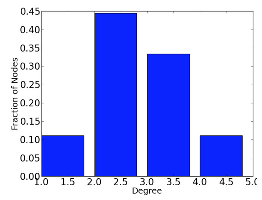
The degree of a node in an undirected graph is the number of neighbors it has.

The degree distribution of a graph is the probability distribution of the degrees over the entire network.

degrees = G.degree()
degree_values = sorted(set(degrees.values()))
histogram = [list(degrees.values()).count(i)/float(nx.number_of_nodes( G)) \
            for i in degree_values]

import matplotlib.pyplot as plt

plt.bar(degree_values,histogram)
plt.xlabel('Degree')
plt.ylabel('Fraction of Nodes')
plt.show()

From University of Michigan, Python for Data Science Coursera Specialization

6.1. Preferential Attachment Model¶

The degree distribution of a graph is the probability distribution of the degrees over the entire network.

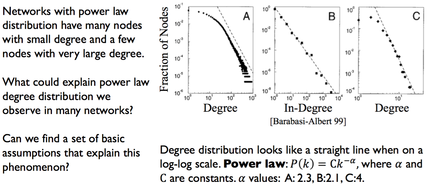
Many real networks have degree distributions that look like power laws (𝑃𝑘 =C𝑘^-a).

Networks with a power law distribution have many nodes with small degree and a few nodes with very large degree.

Models of network generation allow us to identify mechanisms that give rise to observed patterns in real data.

The Preferential Attachment Model produces networks with a power law degree distribution.

From University of Michigan, Python for Data Science Coursera Specialization

nx.barabasi_albert_graph(n, m) returns a network with n nodes. Each new node attaches to m existing nodes according to the Preferential Attachment model.

G = nx.barabasi_albert_graph(1000000,1)
degrees = G.degree()
degree_values = sorted(set(degrees.values()))
histogram = [list(degrees.values().count(i))/float(nx.number_of_node s(G)) \
              for i in degree_values]

import matplotlib.pyplot as plt

plt.plot(degree_values,histogram, 'o')
plt.xlabel('Degree')
plt.ylabel('Fraction of Nodes')
plt.xscale('log')
plt.yscale('log')
plt.show()

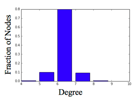
6.2. Small World Model¶

Social networks tend to have high clustering coefficient and small average path length.

Start with a ring of 𝑛 nodes, where each node is connected to its 𝑘 nearest neighbors.

Fix a parameter 𝑝 ∈ [0,1]

Consider each edge 𝑢, 𝑣 . With probability 𝑝, select a node 𝑤 at random and rewire the edge (𝑢, 𝑣) so it becomes (𝑢, 𝑤).

G = nx.watts_strogatz_graph(1000,6,0.04)
degrees = G.degree()
degree_values = sorted(set(degrees.values()))
histogram = [list(degrees.values()).count(i)/float(nx.number_of_node s(G)) \
              for i in degree_values]

import matplotlib.pyplot as plt

plt.bar(degree_values,histogram)
plt.xlabel('Degree')
plt.ylabel('Fraction of Nodes')
plt.show()

From University of Michigan, Python for Data Science Coursera Specialization

Variants of the small world model in NetworkX:

Small world networks can be disconnected, which is sometime undesirable.

nx.connected_watts_strogatz_graph(n, k, p, t) runs watts_strogatz_graph(n, k, p) up to t times, until it returns a connected small world network.

nx.newman_watts_strogatz_graph(n, k, p) runs a model similar to the small world model, sbut rather than rewiring edges, new edges are added with probability 𝑝.

6.3. Link Prediction¶

Given a network, can we predict which edges will be formed in the future?

Typically use these measures as features. And then you would use a classifier, if you have some label data, you would train a classifier and use these measures as features in order to make the prediction.

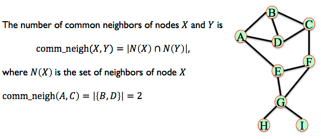
6.3.1. Common Neighbours¶

The number of common neighbors of nodes 𝑋 and 𝑌.

From University of Michigan, Python for Data Science Coursera Specialization

common_neigh = [(e[0], e[1], len(list(nx.common_neighbors(G, e[0], e[1])))) \
                for e in nx.non_edges(G)]

sorted(common_neigh,key=operator.itemgetter(2), reverse = True
print (common_neigh)
# [('A', 'C', 2), ('A', 'G', 1), ('A', 'F', 1),
# ('C', 'E', 1), ('C', 'G', 1), ('B', 'E', 1),
# ('B', 'F', 1), ('E', 'I', 1), ('E', 'H', 1),
# ('E', 'D', 1), ('D', 'F', 1), ('F', 'I', 1),
# ('F', 'H', 1), ('I', 'H', 1), ('A', 'I', 0),
# ('A', 'H', 0), ('C', 'I', 0), ('C', 'H', 0),
# ('B', 'I', 0), ('B', 'H', 0), ('B', 'G', 0),
# ('D', 'I', 0), ('D', 'H', 0), ('D', 'G', 0)]

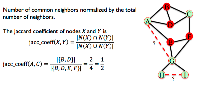
6.3.2. Jaccard Coefficient¶

Number of common neighbors normalized by the total number of neighbors.

From University of Michigan, Python for Data Science Coursera Specialization

L = list(nx.jaccard_coefficient(G))

L.sort(key=operator.itemgetter(2), reverse = True)
print(L)
# [('I', 'H', 1.0), ('A', 'C', 0.5), ('E', 'I', 0.3333333333333333),
# ('E', 'H', 0.3333333333333333), ('F', 'I', 0.3333333333333333),
# ('F', 'H', 0.3333333333333333), ('A', 'F', 0.2), ('C', 'E', 0.2),
# ('B', 'E', 0.2), ('B', 'F', 0.2), ('E', 'D', 0.2), ('D', 'F', 0.2),
# ('A', 'G', 0.16666666666666666), ('C', 'G', 0.16666666666666666),
# ('A', 'I', 0.0), ('A', 'H', 0.0), ('C', 'I', 0.0), ('C', 'H', 0.0),
# ('B', 'I', 0.0), ('B', 'H', 0.0), ('B', 'G', 0.0), ('D', 'I', 0.0),
# ('D', 'H', 0.0), ('D', 'G', 0.0)]

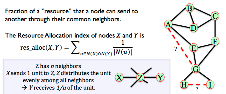
6.3.3. Resource Allocation¶

Fraction of a ”resource” that a node can send to another through their common neighbors. Penalises when common neighbors have high degree of other neighbors as resource will be passed to others. High coefficient when common neighbors have low degree.

From University of Michigan, Python for Data Science Coursera Specialization

L = list(nx.resource_allocation_index(G))

L.sort(key=operator.itemgetter(2), reverse = True)
print(L)
# [('A', 'C', 0.6666666666666666), ('A', 'G', 0.3333333333333333),
# ('A', 'F', 0.3333333333333333), ('C', 'E', 0.3333333333333333),
# ('C', 'G', 0.3333333333333333), ('B', 'E', 0.3333333333333333),
# ('B', 'F', 0.3333333333333333), ('E', 'D', 0.3333333333333333),
# ('D', 'F', 0.3333333333333333), ('E', 'I', 0.25), ('E', 'H', 0.25),
# ('F', 'I', 0.25), ('F', 'H', 0.25), ('I', 'H', 0.25), ('A', 'I', 0),
# ('A', 'H', 0), ('C', 'I', 0), ('C', 'H', 0), ('B', 'I', 0),
# ('B', 'H', 0), ('B', 'G', 0), ('D', 'I', 0), ('D', 'H', 0), ('D', 'G', 0)]

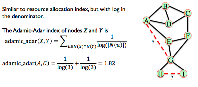
6.3.4. Adamic-Adar Index¶

Similar to resource allocation index, but with log in the denominator.

From University of Michigan, Python for Data Science Coursera Specialization

L = list(nx.adamic_adar_index(G))

L.sort(key=operator.itemgetter(2), reverse = True)
print(L)
# [('A', 'C', 1.8204784532536746), ('A', 'G', 0.9102392266268373),
# ('A', 'F', 0.9102392266268373), ('C', 'E', 0.9102392266268373),
# ('C', 'G', 0.9102392266268373), ('B', 'E', 0.9102392266268373),
# ('B', 'F', 0.9102392266268373), ('E', 'D', 0.9102392266268373),
# ('D', 'F', 0.9102392266268373), ('E', 'I', 0.7213475204444817),
# ('E', 'H', 0.7213475204444817), ('F', 'I', 0.7213475204444817),
# ('F', 'H', 0.7213475204444817), ('I', 'H', 0.7213475204444817),
# ('A', 'I', 0), ('A', 'H', 0), ('C', 'I', 0), ('C', 'H', 0),
# ('B', 'I', 0), ('B', 'H', 0), ('B', 'G', 0), ('D', 'I', 0), ('D', 'H', 0), ('D', 'G', 0)]

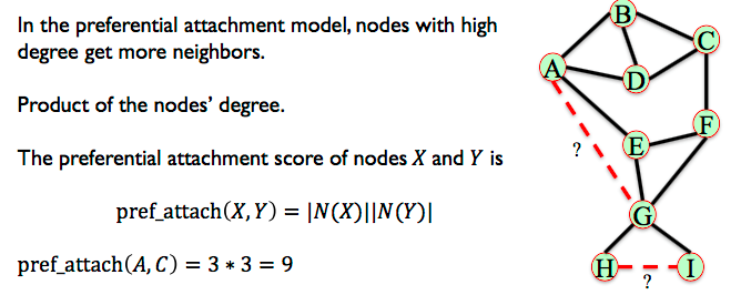
6.3.5. Preferential Attachment¶

In the preferential attachment model, nodes with high degree get more neighbors.

From University of Michigan, Python for Data Science Coursera Specialization

L = list(nx.preferential_attachment(G))

L.sort(key=operator.itemgetter(2), reverse = True)
print(L)
# [('A', 'G', 12), ('C', 'G', 12), ('B', 'G', 12), ('D', 'G', 12),
# ('A', 'C', 9), ('A', 'F', 9), ('C', 'E', 9), ('B', 'E', 9),
# ('B', 'F', 9), ('E', 'D', 9), ('D', 'F', 9), ('A', 'I', 3),
# ('A', 'H', 3), ('C', 'I', 3), ('C', 'H', 3), ('B', 'I', 3),
# ('B', 'H', 3), ('E', 'I', 3), ('E', 'H', 3), ('D', 'I', 3),
# ('D', 'H', 3), ('F', 'I', 3), ('F', 'H', 3), ('I', 'H', 1)]

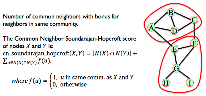
6.3.6. Community Common Neighbors¶

Some measures consider the community structure of the network for link prediction. Assume the nodes in this network belong to different communities (sets of nodes). Pairs of nodes who belong to the same community and have many common neighbors in their community are likely to form an edge.

Number of common neighbors with bonus for neighbors in same community.

From University of Michigan, Python for Data Science Coursera Specialization

# add node attribute to differentiate between communities
G.node['A']['community'] = 0
G.node['B']['community'] = 0
G.node['C']['community'] = 0
G.node['D']['community'] = 0
G.node['E']['community'] = 1
G.node['F']['community'] = 1
G.node['G']['community'] = 1
G.node['H']['community'] = 1
G.node['I']['community'] = 1


L = list(nx.cn_soundarajan_hopcroft(G))

L.sort(key=operator.itemgetter(2), reverse = True) print(L)
# [('A', 'C', 4), ('E', 'I', 2), ('E', 'H', 2), ('F', 'I', 2),
# ('F', 'H', 2), ('I', 'H', 2), ('A', 'G', 1), ('A', 'F', 1),
# ('C', 'E', 1), ('C', 'G', 1), ('B', 'E', 1), ('B', 'F', 1),
# ('E', 'D', 1), ('D', 'F', 1), ('A', 'I', 0), ('A', 'H', 0),
# ('C', 'I', 0), ('C', 'H', 0), ('B', 'I', 0), ('B', 'H', 0),
# ('B', 'G', 0), ('D', 'I', 0), ('D', 'H', 0), ('D', 'G', 0)]

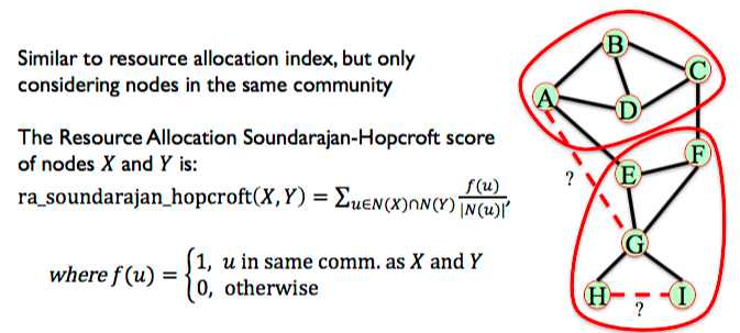
6.3.7. Community Resource Allocation¶

Similar to resource allocation index, but only considering nodes in the same community

From University of Michigan, Python for Data Science Coursera Specialization

L = list(nx.ra_index_soundarajan_hopcroft(G))

L.sort(key=operator.itemgetter(2), reverse = True)
print(L)
# [('A', 'C', 0.6666666666666666), ('E', 'I', 0.25),
# ('E', 'H', 0.25), ('F', 'I', 0.25), ('F', 'H', 0.25),
# ('I', 'H', 0.25), ('A', 'I', 0), ('A', 'H', 0), ('A', 'G', 0),
# ('A', 'F', 0), ('C', 'I', 0), ('C', 'H', 0), ('C', 'E', 0),
# ('C', 'G', 0), ('B', 'I', 0), ('B', 'H', 0), ('B', 'E', 0),
# ('B', 'G', 0), ('B', 'F', 0), ('E', 'D', 0), ('D', 'I', 0),
# ('D', 'H', 0), ('D', 'G', 0), ('D', 'F', 0)]